Difference between revisions of "Walkthrough on GUI based tilt series alignment"
(→Data) |
|||
| Line 4: | Line 4: | ||
We use a binned version of the first tilt series from the EMPIAR entry 10164, depicting a set of virus like particles (VLP). Visit the course materials to access the tilt series or download it directly from EMPIAR. You can also follow this tutorial using your own data. | We use a binned version of the first tilt series from the EMPIAR entry 10164, depicting a set of virus like particles (VLP). Visit the course materials to access the tilt series or download it directly from EMPIAR. You can also follow this tutorial using your own data. | ||
| − | |||
= Creating an alignment workflow= | = Creating an alignment workflow= | ||
Revision as of 17:14, 5 August 2021
Dynamo includes a package for automated alignment and reconstruction of tilt series. This walkthrough guides users through a series of steps on how to use it in GUI-based mode. The walkthrough on command line based tilt series alignment shows how to operate this procedure through the command line.
Contents
Data
We use a binned version of the first tilt series from the EMPIAR entry 10164, depicting a set of virus like particles (VLP). Visit the course materials to access the tilt series or download it directly from EMPIAR. You can also follow this tutorial using your own data.
Creating an alignment workflow
Start the alignment GUI by typing the command dtsa (short form of dynamo_tilt_series_alignment) into the Dynamo command line:
dtsa
A pop-up window appears. Click on "create a new workflow":
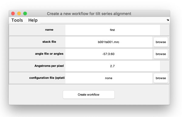
Here, the input data for the workflow (tilt series, angles, ...) is introduced:
The option configuration file is used to pass information on possible tilts that should be discarded. Here, we leave this option untouched. Press on create workflow.
GUI description
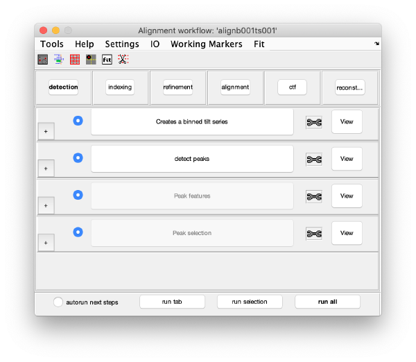
The GUI guides the process of creating a set of working markers in the tabs detection, indexing and refinement. These markers are then used to create the aligned tilt series in the alignment tab. There is further the option to estimate and correct the CTF (using wrappers of ctfffind4 and imod) and to finally create the 3D reconstructions of the tomographic data.
Alignment GUI Controls
The GUI has different pre-defined areas. Starting from top to bottom, you can find a toolbox with the options: Tools, Help, Settings, IO, Working Markers and Fit. These tools contain different visualization methods and also let you customize general settings. The option Settings > edit[general] for example lets you adjust again the pixel size and different acquisition parameters such as Cs etc. Here we use the default settings.
Under the toolbox, we find several icons: dmarkers, occupancy plot, gold bead gallery, gold bead targeting, fitting and marker selection. Their functionalities will be explained in the following.
Execution Areas
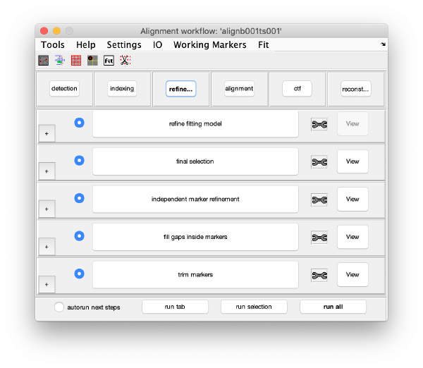
In the GUI, right below the icons, we can find six execution areas: detection, indexing, refinement, alignment, ctf, reconstruction. Each of them comprises a set of steps that can be executed sequentially. Sequential execution is the natural way of proceeding; but steps can be visited in any order, i.e., a step can be re-executed in a later moment after updating its information.
Steps
Each execution area has one or more steps. Steps need to be open (letters highlighted in black, not grey) to be executed. They become open when the required input(s) is ready to be processed. The required input(s) can be provided by users or computed and stored in a previous step of this alignment workflow. When a step is under execution, its pushbutton becomes green. Input parameters are edited by clicking the plus button on the left.
At the right side of each of the steps, a tool icon is located. The tool icon can be right-clicked to provide a pop-up menu with specific tools for each step. There are also some common tools for all the steps which handle the inspection and listing of input and output items generated by the step.
Next to the tool icon, there is a View pushbutton. The View pushbutton provides specific tools to visualize and inspect the results of each step.
Detection
The goal of this step is to find the positions of the gold bead projections in the tilt series. To do that, Dynamo cross correlates each micrograph against a 2D model of the gold bead and then locate the cross correlation peaks, which provide putative positions for actual projections of gold beads. Further analysis of these peaks will determine which ones correspond to actual gold bead projection (peak feature and peak selection).
Visualization matrix
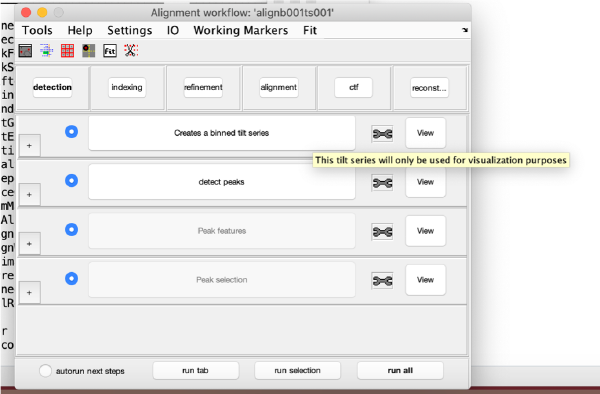
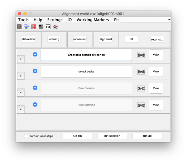
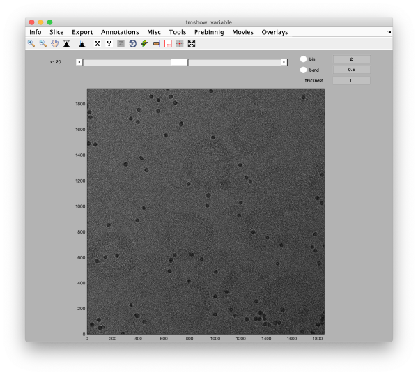
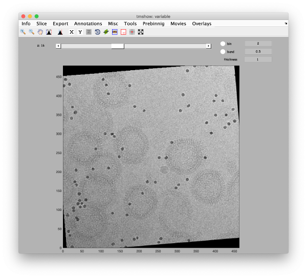
This step just creates a binned version of the tilt series stack to accelerate visualizations that will be invoked in a later point. If you click on the box standing on the left of creates a binned tilt series button with a + symbol, an option box appears, indicating the default binning factor which is 2. This parameter can be changed by users. Binning factor 2 in Dynamo is equivalent to a binning factor of 4 in IMOD. Click on creates a binned tilt series button to create a binned tilt series stack. Rightclick on View button to visualize the newly binned tilt series stack in tmshow. In the tmshow window, visualization parameters as binning, band and thickness can be adjusted if needed.
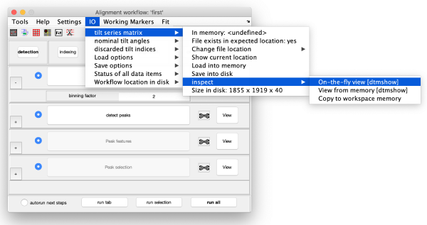
Now, we are going to measure the diameter of the gold beads precisely in tmshow in the original (unbinned) tilt series data. To do that, press the IO in the upper toolbox of the alignment workflow GUI, then go to tilt series matrix > inspect > On-the-fly view [dtmshow]. The tmshow window opens, adjust contrast if necessary for better visualization.
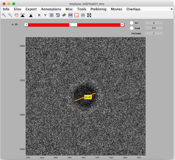
Zoom in a gold bead by holding the shift key and scrolling up your mouse wheel. Adjust the visualized region by holding the shift key again and dragging with right mouse click on tmshow window.
Once you have located the gold bead of interest, click on the ruler icon at the top toolbox to activate length measurements on the displayed image data. Draw a line across the gold bead, and the length of the line appears in pixels, which correspond to the gold bead diameter. In this case, the length of this line should be 32 pixel aprox.
Detection of gold beads
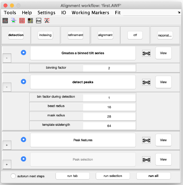
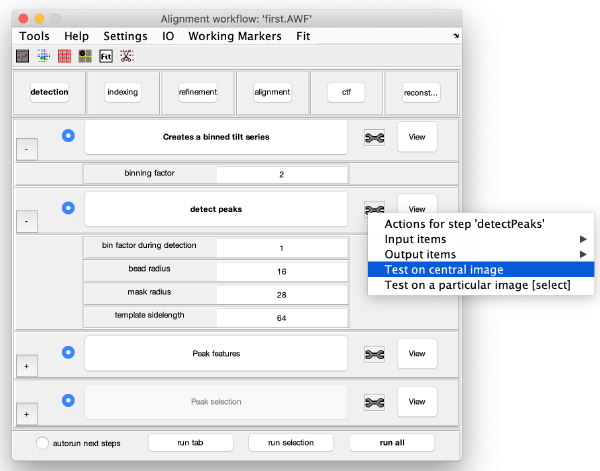
Here we provide the size of the gold beads. The measured diameter of the gold beads is 32 pixels in the original image, therefore its radius is 16 pixels. We introduce the bead radius and some other parameters (see screenshot) to create an accurate initial gold bead template (here, the binning is just used internally for quick and robust bead detection).
After pressing the button detect peaks, Dynamo creates a raw cross-correlation matrix based on the initial template which is binary and extracts 300 cc-peaks by default. Then, the extracted peaks are averaged to create a refined template. The refined template is used to compute a refined cc-matrix from which 300 peaks are extracted and used as initial working markers. Once the detect peaks button turns black bold, the computation is finished. Right click on the view area of the step to access the different visualisation options.
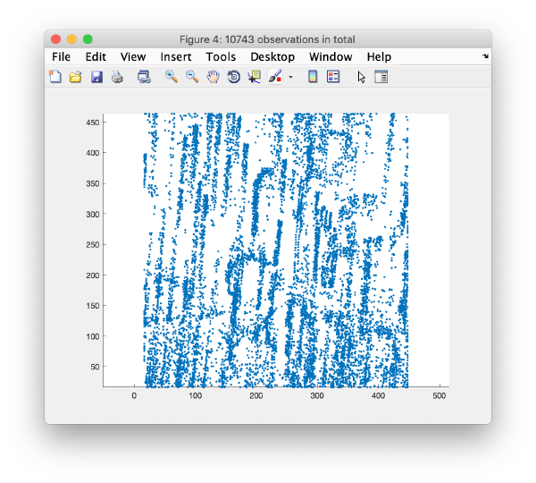
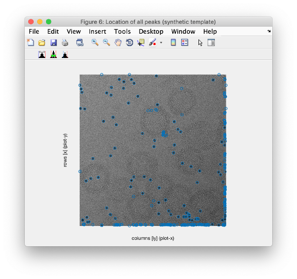
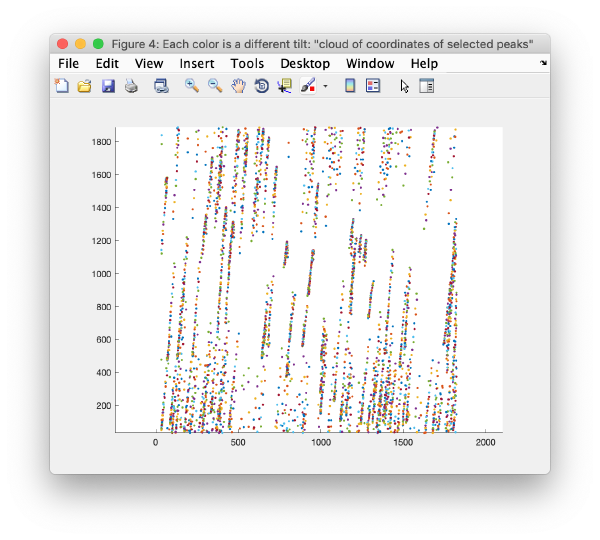
This view shows the overlaid sum of the x,y coordinates of all cc peaks from all micrographs in the tilt series.
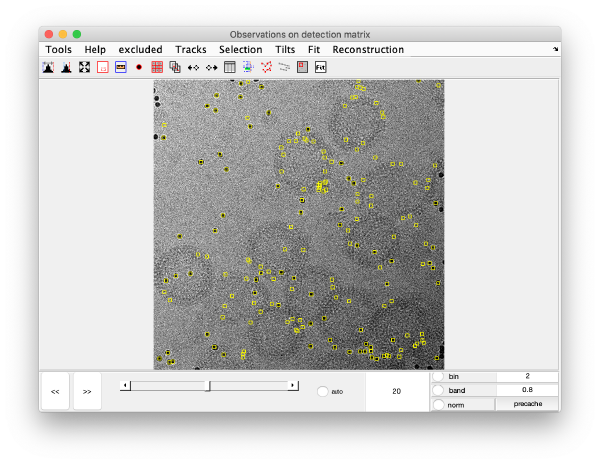
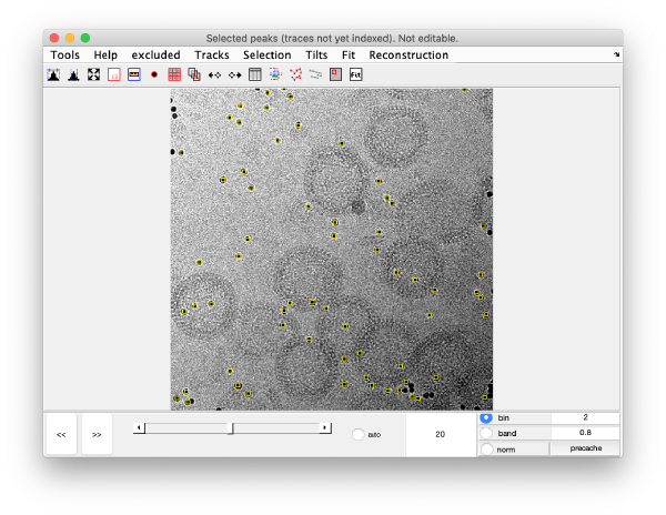
We can also check the positions of all the detected spots on each micrograph:
This GUI does not allow for edition of the markers. Tip: enable auto option at the bottom center of the visualization GUI to facilitate tilt series visualization.
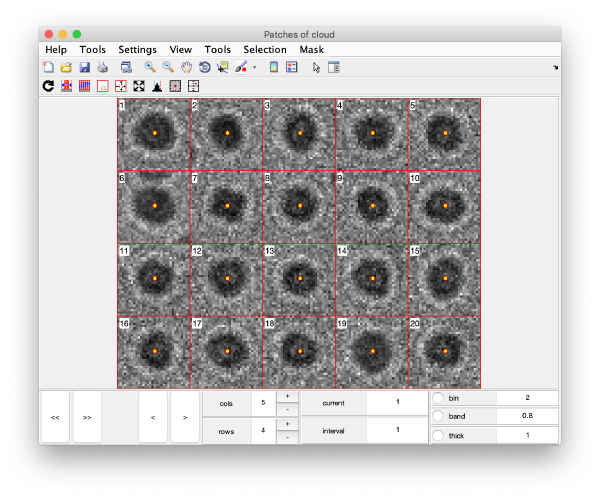
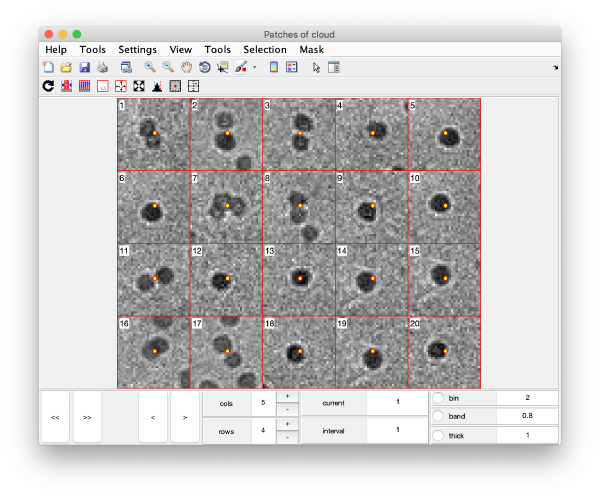
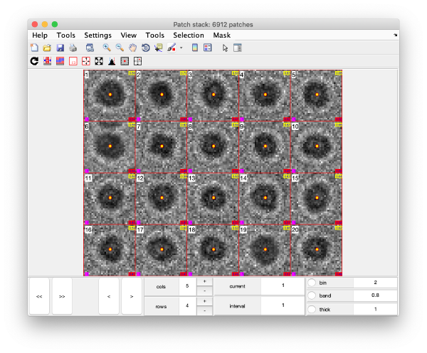
The neighbourhood of cross correlation peaks can be visualised individually as 2D patches from the tilt series image data:
This visualization is normally a good gauge on how the detection procedure has worked. The example below would be an example of detection procedure carried with wrong search parameters
Note that you have the option of testing your parameters against a single image before launching a full detection procedure. Right-click on the tool icon on the right side of detect peaks pushbutton.
Computation of observation features
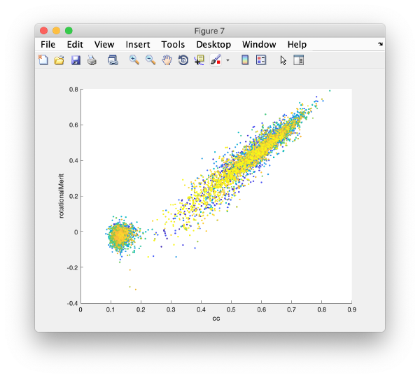
At this stage, the observed cross correlation peaks are analysed. A merit figure is assigned to each peak based on a rotational merit that measures its rotational symmetry. Press the button Peak features to compute the rotational symmetry of the current working markers. The working markers that do not meet rotational symmetry will be discarded. The results can be depicted on patches representing individual gold beads:
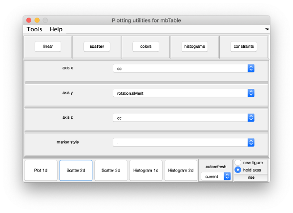
or extracting properties of the whole data set.
Selection of best gold beads
The population with the best markers is automatically selected by clicking on Peak selection. The results can be inspected again in a plot
or in the micrographs themselves:
Indexing
The goal of this execution area is to find trails of gold beads, i.e., we connect the observations from different micrographs that correspond to the same gold bead. All the steps in this area will constantly update a set of working markers.
Rough Alignment
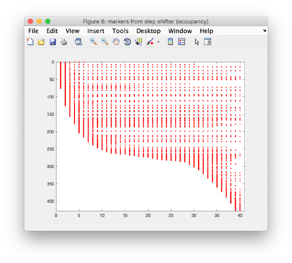
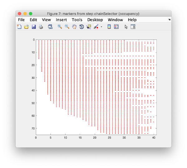
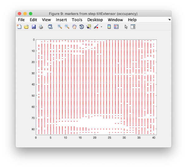
In this step, micrographs are compared pair-wise. For each couple, we look for the relative shifts that generate the most matches of cross-correlation peaks between one micrograph and the next one. This procedure induces trails of matched pairs of observations of variable length along the tilt series. The scheme that depicts which trails have representatives in which tilts is called occupancy graph
Note that these trails are very lacunary and do not conserve the identity of a trail; whenever a trail that represents an actual 3d marker gets interrupted, the same 3d marker might generate a different trail in other tilts.
Keep long chains
Click on keep long chains to select the longest trails, which will then be used to generate a 3d model of the markers:
Note that from this step onwards, the toolbox of each step offers the possibility to revert the current markers to the output generated at that state. Thus, if further processing of the markers in a later step leads you to loose a good marker set, you can always come back to this point.
Iterative reindexing
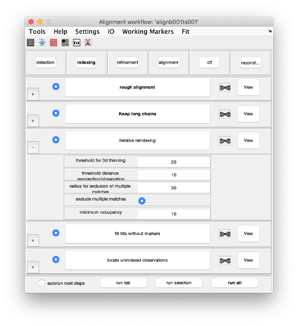
The 3d model is projected on each micrograph. Observations that are closest (and below a distance threshold) to each reprojection are assigned to the corresponding 3d marker. This refines the 3d model, and the process is iterated till no further improvement occurs (or till a maximum of ten iterations is reached). Keep the default parameters and click on iterative reindexing.
Tilt gap filling
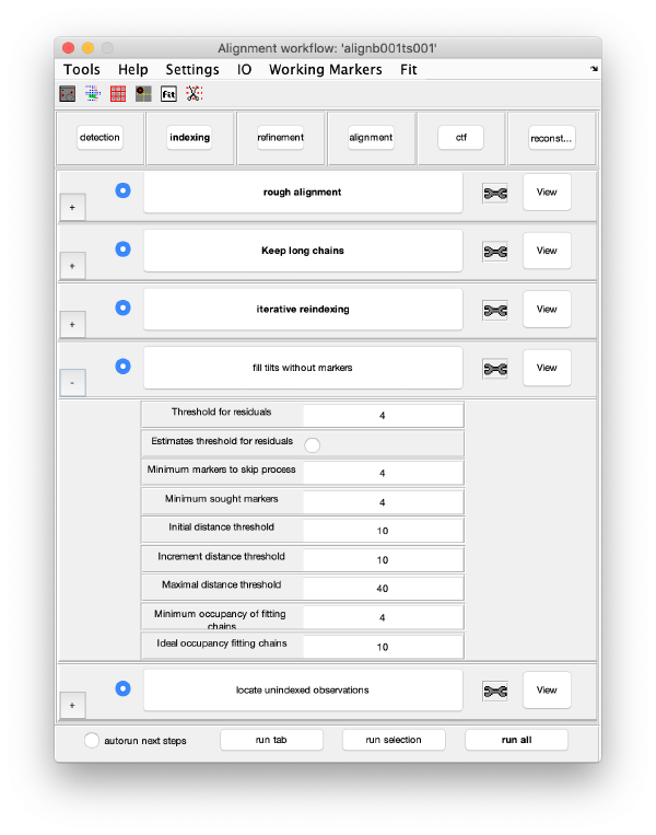
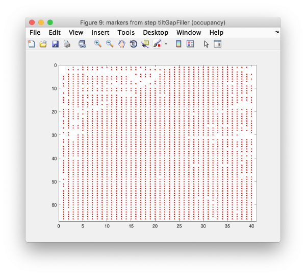
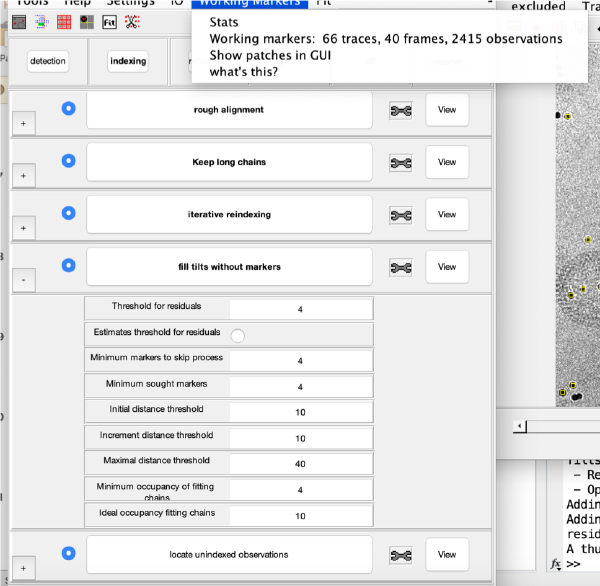
Here, potential tilts with too few (or zero) markers can be rescued. The cloud of observations found on that micrograph will be compared to the cloud or reprojections generated by the current model. Click on fill tilts without markers.
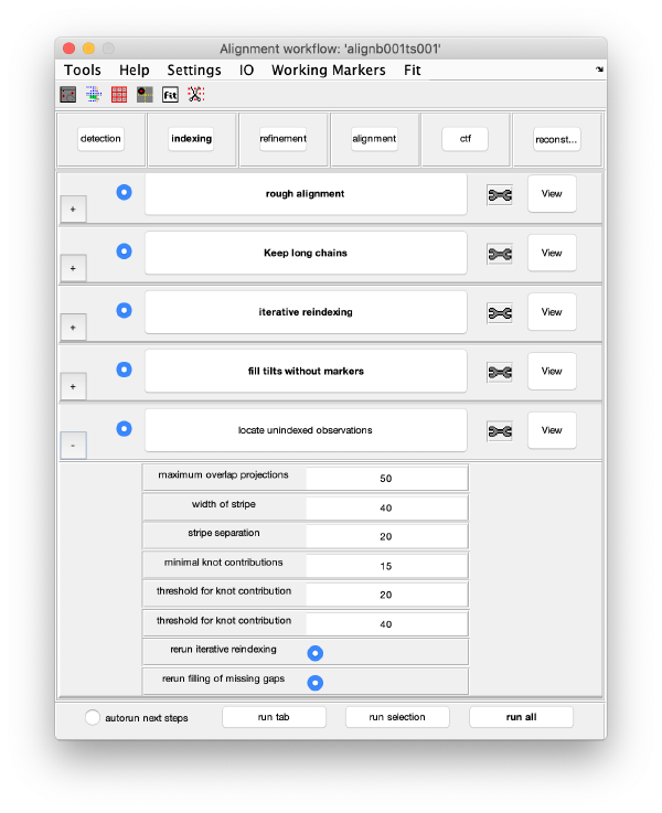
Trail extension
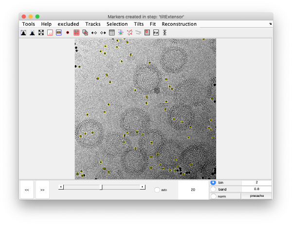
This step aims at locating trails that have been excluded by previous steps of the alignment procedure, or that were never detected as trails because previous, lesser quality stages of the 3d model were not able to analyse the observations correctly.
Note that newly added trails have empty spaces in the central area, they are likely to be gold beads located far away from the tilt axes and which get into the field of view only for high tilts.
Refinement
This area refines the positions of the gold beads. We will run all steps of this area by pressing on a single button (the run this tab option at the bottom of the GUI). The button will remain green while the different steps are computed.
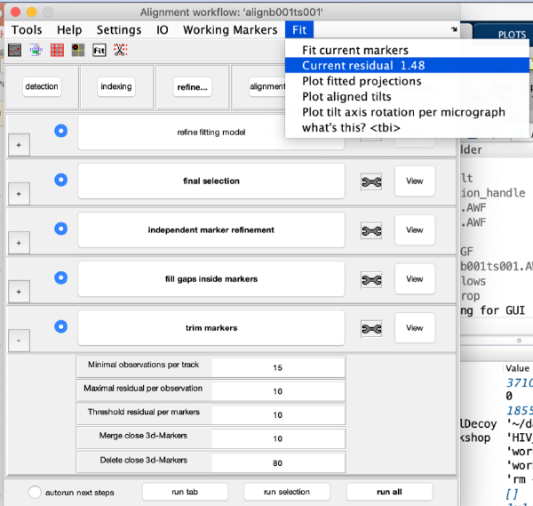
Check the current refinement error:
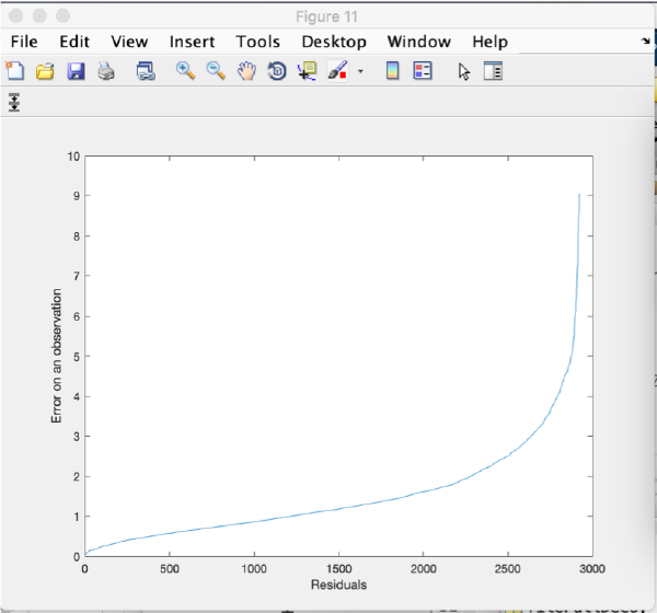
Optionally, we can use the scissors icon to "trim" observations (or full markers) with too high residuals. Click on the scissor icon. A window pops up with options to set different thresholds. Click on Tools and then Show residuals per observation:
You get a plot with the residuals for each observation ordered by the value of the residual. You can use this plot to estimate the residual distribution and to manually adapt the residual thresholds, if necessary.
Alignment
The final step of the alignment procedure is to create the aligned tilt series using the coordinates of the markers that were optimized until now.
Fix the markers
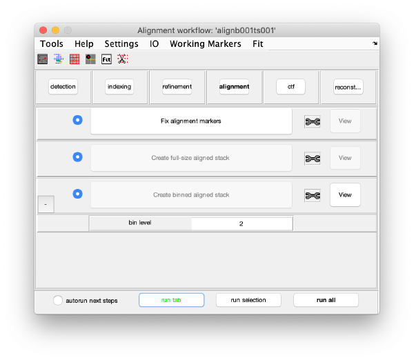
Here we freeze the final version of the working markers and create a marker file that will define all subsequent steps of alignment and reconstruction. Click on fix alignment markers.
Align the tilt series
We then proceed to the alignment task itself, generating full resolution aligned tilt series. We also have the option to generate a binned version of the aligned tilt series that can be used for quick visualization or to create binned reconstructions in the next steps. Click on Create full-size aligned stack and Create binned aligned stack. For a quick assessment, open the binned stack in tomoshow:
A quick way to gauge the quality of the alignment is by checking that the beads move nicely horizontally over all tilts.
CTF
In this GUI, CTF estimation and correction are done using CTFFIND4 and IMOD's ctfphaseflip. This part will not be used in the workshop.
Reconstruction
Binned reconstruction
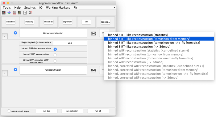
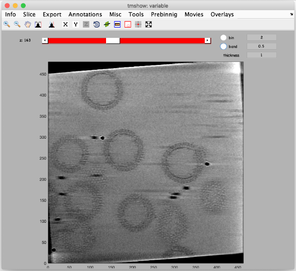
Click on binned reconstruction to create a binned tomogram using the previously created binned aligned tilt series. Adapt the tomogram height if necessary (the tomogram center is automatically located at the center of the 3d reconstruction of the aligned stack). Select binned SIRT-like reconstruction to generate a high contrast tomogram. Run the step binned reconstruction and visualize the resulting binned SIRT-like tomogram:
Full sized reconstruction
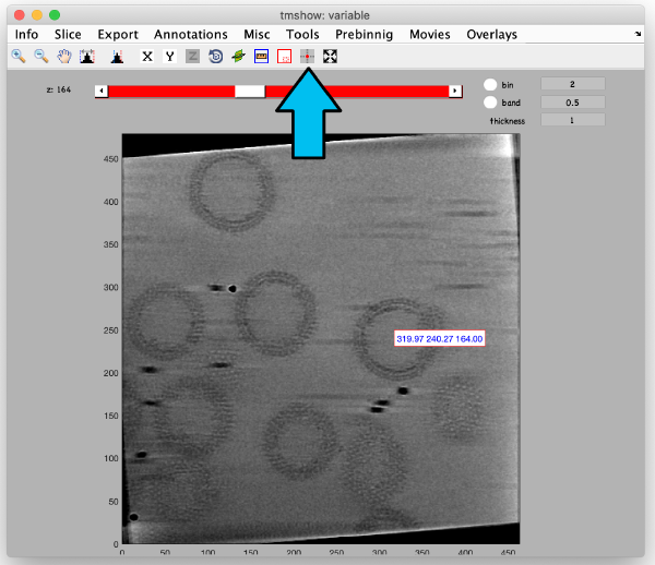
The full sized reconstruction is the one you will be using for later image processing steps that require the highest resolution possible (e.g., subtomogram averaging refinements). It can be created related to a coordinate directly read from the binned tomogram. This feature is useful to create reconstructions localised on an area of interest. In this tutorial, we will focus on one of the VLPs, resulting in a tomogram containing just one VLP. First, use the pin tool to select a point on the binned reconstruction. We use the previously opened binned SIRT-like tomogram for this:
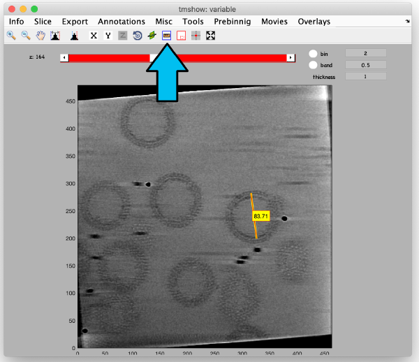
We check the size of the structure by using the measuring tool:
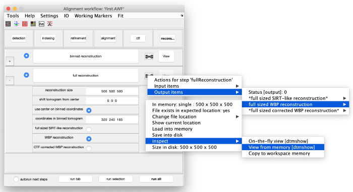
Before generating the final localized tomogram, we need to set some parameters. We take the measured distance of 83 pixels and compensate for the binning factor of two, leading to 83*2*2=332 pixels. For the dimensions of the tomogram we add some spare space and define the x,y and z length to be 500 pixels. Select use center of binned coordniates and enter the values we measured before with the pin tool. Select WBP reconstruction and run the step full reconstruction. Use the inspection tools to fetch the result:
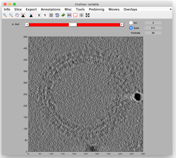
As it is a WBP reconstruction, it is much noisier than the corresponding area in the SIRT-like tomogram. Adjust the contrast, lowpass filter and thickness to increase the signal:

